about me
- applied econometrics, computer science (Master)
- economic theory (PhD)
- software for statistics and economtrics
- user-developer with various packages and with GAUSS, Matlab, Python
- scipy.stats
- statsmodels
- "self-taught statistician"
about statsmodels
- precursor: scipy.stats.models
- 7 years of development
- started with GSOC Skipper Seabold
- slow and steady growth since then
- GSOC Chad Fulton statespace models
- open source, BSD licensed
- ~ 130,000 LOC of Python (including some Cython)
Brief Overview - Time Series Analysis in Statsmodels
- Data Handling through Pandas
- statistics
- acf, pacf
- filters, seasonal decomposition
- hypothesis tests: unit root, Granger causality
- ARMA, ARIMAX
- VAR (vector autoregressive models)
- new statespace models
- SARIMAX
- ...
- postestimation: predict, impulse response, hypothesis testing
two GSOC projects in 2016 for TSA
%matplotlib inline
import datetime

import numpy as np
import pandas as pd
import matplotlib.pyplot as plt
from dateutil.relativedelta import relativedelta
import seaborn as sns

import statsmodels.api as sm
import statsmodels.formula.api as smf
from statsmodels.tsa.stattools import acf
from statsmodels.tsa.stattools import pacf
from statsmodels.tsa.seasonal import seasonal_decompose
#plt.interactive(False)   # otherwise interactive(False)
El Nino temperature data
from statsmodels.datasets.elnino import load_pandas

datadf = load_pandas()
datadf.data
temperature = np.asarray(datadf.data.iloc[:, 1:]).ravel()
nobs = len(temperature)
index = pd.date_range("1950-01-01", periods=nobs, freq='MS')
months = np.tile(np.arange(12), nobs // 12)
df_el = pd.DataFrame({'temperature': temperature, 'month': months}, index=index)
df_el.tail()
ax = df_el['temperature'].plot()
ax.figure.set_size_inches(12, 8)
ax.set_title('Temperature', fontsize=18)

ax = df_el['temperature'].iloc[-12*5:].plot(style='-o')
ax.figure.set_size_inches(12, 8)
_ = ax.set_title('Temperature', fontsize=18)

res_ols = sm.formula.ols('temperature ~ C(month)', df_el.iloc[:-3*12]).fit()
predicted = res_ols.predict(df_el.iloc[-3*12:])
fitted = res_ols.fittedvalues.loc['2005-12-01':]  # 5 years
ax = df_el['temperature'].iloc[-12*5:].plot(style='-o')
ax.figure.set_size_inches(12, 6)
fitted.plot(lw=2, color='r')
predicted.plot(lw=2, color='r')
ax.vlines(predicted.index[0], lw=4, alpha=0.25, *ax.get_ylim())
_ = ax.set_title('Constant Seasonal Pattern - fitted and predicted', fontsize=18)

ax = res_ols.resid.iloc[-5*12:].plot(style='-o',figsize=(12,8))
_ = ax.set_title('Residuals insample', fontsize=18)

_ = cfplot(res_ols.resid, lags=36)

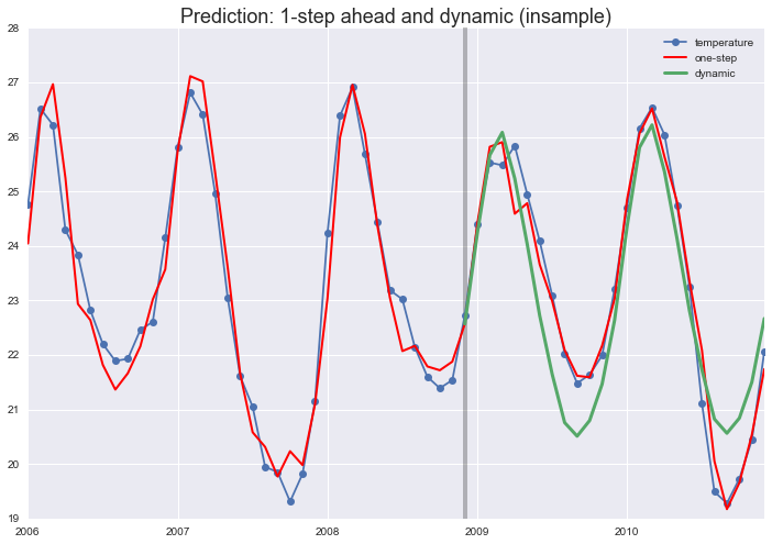
import patsy
y, x = patsy.dmatrices('temperature ~ C(month)', df_el, return_type='dataframe')
res_arma = sm.tsa.ARMA(y, order=(2, 1), exog=x.iloc[:, 1:]).fit()
print(res_arma.summary())
pred_dynamic = res_arma.predict(start='2008-12-01', end='2010-12-01', exog=res_arma.model.exog[-3*12:, 1:], dynamic=True)
fitted = res_arma.fittedvalues
Short term and long term forecasts
Summary ARMAX
y = X b + e, e ~ ARMA(p, q)
use explanatory variables X to model stable, systematic part
- seasonal patterns: dummies, splines, fourier polynomials
- trend: linear, polynomial, or piecewise
- other effects: dummies for special events, outliers
- explanatory variables: related series that help in prediction, (need forecasts for those, or use lagged values)
use ARMA to improve short term forecasting
- e = y - X b
- use the additional information that is left after systematic part has been removed
- assumes what is left over is stationary
Stationarity
A time series is stationary if the distribution of the observations does not depend on time.
Often only mean, variance and autocovariance stationarity is relevant
no persistence: shocks or disturbances have not long term effect
mean reversion: the long term forecast moves to the mean of the series
Random Walk y(t) = y(t-1) + e(t)
The best forecast at time t $\hat{y}(t+1) = y(t)$ and $\hat{y}(t+h) = y(t)$
Tomorrow is like today.
seasonal y(t) = y(t - s) + e(t)
Tomorrow is like the same day last week (month, year)
full persistence: every shock stays forever
y(t) is integrated, the differenced series is stationary
substituting back in
$y(t) = y(0) + \sum_{i=1}^{t} e(t-i)$
SARIMAX without X
SARIMAX(endog, exog=None, order=(1, 0, 0), seasonal_order=(0, 0, 0, 0), trend=None, ...)
endog is endogenous, dependent variable (statsmodels econometrics history)
exog are eXogenous, independent, explanatory variables
order (p, d, q) is regular ARIMA
seasonal_order (P, D, Q, s) is seasonal ARIMA with season length s
example: SARIMA((1, 0, 0), (1, 0, 0, 12) only AR terms
$(1 - a_1 \hspace{2mm} L) (1 - A_1 \hspace{2mm} L^{12}) y_t = y_t - a_1 \hspace{2mm} y_{t-1} - A_1 \hspace{2mm} y_{t-12} + a_1 \hspace{2mm} A_1 \hspace{2mm} y_{t-13}$
$y_t = a_1 \hspace{2mm} y_{t-1} + A_1 \hspace{2mm} y_{t-12} - a_1 \hspace{2mm} A_1 \hspace{2mm} y_{t-13} \hspace{2mm} + ...$
Model Selection and Automatic Forecasting
Hyndman has several supporting functions in R, auto.arima
statsmodels doesn't have much ready made and automatic
Amount of Differencing
(standard maximum likelihood methods do not apply)
commonly based on unit root or stationarity tests
Lag lengths, p, q, P, Q
loop over set of lag lengths and choose the model
minimize AIC, BIC, or maximize out-of-sample forecast performance.
Outliers, ...
dummies for outlier observation, trend breaks, ...
Example: Forecasting Bus Riders
see blog post and notebook for details
http://www.seanabu.com/2016/03/22/time-series-seasonal-ARIMA-model-in-python/
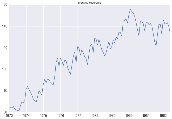
seas = seasonal_decompose(df['riders'])
fig = seas.plot()
fig.set_size_inches(12,8)

mod = sm.tsa.statespace.SARIMAX(df.riders, order=(0,1,0), seasonal_order=(1,1,1,12), trend='n')
results = mod.fit()
results.summary()
df['forecastd'] = results.predict(start=102, end=114, dynamic=True)
df['forecastnd'] = results.predict(start=102, end=114, dynamic=False)
df[['riders', 'forecastd', 'forecastnd']].loc['1979-01-01':].plot(figsize=(12, 8), color='brk', lw=3, alpha=0.5)
plt.savefig('images/ts_df_predict.png', bbox_inches='tight')

SARIMAX and transformation
back to the initial plot
df_air = pd.read_csv('AirPassengers.csv', index_col=0)
di = pd.date_range("1949-01-01", periods=144, freq='MS')
df_air.set_index(di, inplace=True)
del df_air['time']
df_air.tail()
df_air.plot(figsize=(12,6))
plt.savefig('air_passenger.png', bbox_inches='tight')

air_log = np.log(df_air['AirPassengers'])
air_log.plot(figsize=(12,6))

Rolling Standard Deviation - orginal versus log transformed
fig, (ax1, ax2) = plt.subplots(2, 1, sharex=True, figsize=(12,6))
_ = df_air['AirPassengers'].rolling(12).std().plot(ax=ax1)
_ = air_log.rolling(12).std().plot(ax=ax2)

Rolling Standard Deviation - Box-Cox transformed
from scipy import special
ax = special.boxcox(df_air['AirPassengers'], -0.2).rolling(window=12).std().plot(figsize=(12,6))

def box_cox_rolling_coeffvar(box_cox_param, endog, freq):
    """helper to find Box-Cox transformation with constant standard deviation

    returns RLM results instance
    """
    roll_air = special.boxcox(endog, box_cox_param).rolling(window=freq)
    y = roll_air.std()
    m = roll_air.mean()
    x = sm.add_constant(m)
    res_rlm = sm.RLM(y, x, missing='drop').fit()
    return res_rlm

endog = df_air['AirPassengers']
freq = 12
tt = [(lam, box_cox_rolling_coeffvar(lam, endog, freq).pvalues[1]) for lam in np.linspace(-1, 1, 21)]

tt = np.asarray(tt)
print(tt[tt[:,1].argmax()])
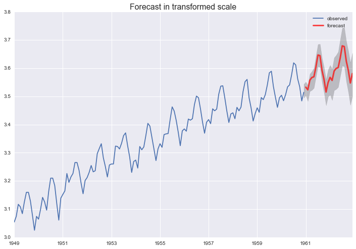
SARIMAX((1, 1, 1), (0, 1, 1, 12)) of transformed series
air_t = special.boxcox(df_air['AirPassengers'], -0.2)
res_s = sm.tsa.SARIMAX(air_t, order=(1, 1, 1), seasonal_order=(0, 1, 1, 12)).fit()
res_s.summary().tables[1]
max_ar, max_ma = 3, 3
aic_full = pd.DataFrame(np.zeros((max_ar, max_ma), dtype=float))

# Iterate over all ARMA(p,q) models with p,q in [0,1, 2]
for p in range(max_ar):
    for q in range(max_ma):
        if p == 0 and q == 0:
            continue

        # Estimate the model with no missing datapoints
        mod = sm.tsa.statespace.SARIMAX(air_t, order=(p,1,q), seasonal_order=(0, 1, 1, 12), trend='c', enforce_invertibility=False)
        try:
            res = mod.fit()
            aic_full.iloc[p,q] = res.aic
        except:
            aic_full.iloc[p,q] = np.nan

print('min at ', np.asarray(aic_full).argmin())
aic_full
pred = res_s.get_prediction(start='1960-12-01', end='1962-12-01')
pred_ci = pred.conf_int()

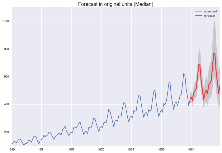
Transform forecast to original scale
pred_ci_orig = special.inv_boxcox(pred.conf_int(), -0.2)
forecast = special.inv_boxcox(pred.predicted_mean, -0.2)
ax = df_air['AirPassengers'].plot(label='observed')
ax.figure.set_size_inches(12, 8)
forecast.plot(ax=ax, label='forecast', lw=3, alpha=.7, color='r')
ax.fill_between(pred_ci_orig.index,
                pred_ci_orig.iloc[:, 0],
                pred_ci_orig.iloc[:, 1], color='k', alpha=.15)
ax.set_title('Forecast in original units (Median)', fontsize=16)
plt.legend()
plt.savefig('images/airpassenger_forecast.png', bbox_inches='tight')

mod_ucarima = sm.tsa.UnobservedComponents(air_t, 'lltrend', seasonal=12, autoregressive=4)
res_ucarima = mod_ucarima.fit(method='powell', disp=0)
print(res_ucarima.summary())
fig_uc = res_ucarima.plot_components()
fig_uc.set_size_inches(12, 8)

pred_uc = res_ucarima.get_forecast(steps=24)
pred_ci = pred.conf_int()
#pred_uc.predicted_mean
References
documentation
http://www.statsmodels.org/dev/tsa.html
http://www.statsmodels.org/dev/statespace.html
http://www.statsmodels.org/dev/examples/index.html
blog posts
http://tomaugspurger.github.io/modern-7-timeseries.html Pandas usage
http://www.seanabu.com/2016/03/22/time-series-seasonal-ARIMA-model-in-python/
http://www.analyticsvidhya.com/blog/2016/02/time-series-forecasting-codes-python/
I will clean up notebook during weekend